Starting out with neural networks

In this post I'll talk about the process I went through when starting to explore the strange and wonderful world of recurrent neural networks

It all started with Dan Hon. You may know of Dan from his rather amusing posts, including “I trained an A.I. to generate British placenames”, “I trained an A.I. to generate ICD-10 codes”, English idioms, Ask MetaFilter, and more. On Monday I was coming home from London on the train, and Dan popped up on Twitter with his latest creation: “I trained an A.I. to write Star Trek episode titles”.

Reading through the article, I was struck by the contrast of generating new words and phrases with a neural network, and the work that I’ve been involved with lately - a lot of which revolves around standardisation. In a giant leap that only really made sense at the time, I started wondering what would happen if I deliberately went against the concept of standardisation, and instead try to generate some weird and wonderful new things for myself? I spent the rest of that evening reading, learning, and doing, and wanted to capture some of that in case others are interested in playing with A.I. themselves. The audience for this is intended as other complete beginners, and it will inevitably be filled with over-simplification and errors in various areas. I’ve also tried to explain some basic terms as we go along, in case people are reading this who perhaps have less development experience.

Background reading

Whilst you’re probably itching to get stuck into doing, before we get there I wanted to introduce a couple of pieces of background reading to explain a bit more about the concepts behind all of this.

As you may be able to deduce from my rather short-lived career in this area (3 days and counting), I’m perhaps not the leading authority on neural networks. I therefore won’t be digging into the complexities, mostly because I don’t understand nearly enough to explain it correctly yet. Things that helped me to understand some of the basic concepts include the following:

I started off with the rather obvious: searching for posts that would give me a “simple” understanding. These were pretty useful in getting to grips with some of the core concepts. Now, heads up, you’re going to see a lot of formulae and code in the following links, but bear with me. I did A-Level Maths and Statistics but have forgotten everything, and all of the formulae went completely over my head. Read to understand concepts, but don’t worry at this point if you don’t follow everything (we can still make stuff!).

• How to build a simple neural network in 9 lines of Python code by Milo Spencer-Harper
• A Neural Network in 11 lines of Python (Part 1) by Andrew Trask (linked by Milo)
• How to build a multi-layered neural network in Python by Milo Spencer-Harper

At this point I wanted to know more about the recurrent element that Dan had mentioned, so I started searching for “recurrent neural networks” and “LSTM networks” (Long short-term memory, by the way, and not the Liverpool School of Tropical Medicine). These all had some good elements:

• Understanding LSTM Networks by Christopher Olah
• Recurrent Neural Networks by TensorFlow - this was useful in understanding some of the config options that I was later able to tweak in my work, and how they affected the process.
• The Unreasonable Effectiveness of Recurrent Neural Networks by Andrej Karpathy - some really nice examples in here
• A Beginner’s Guide to Recurrent Networks and LSTMs by Deeplearning4j

Phew. That’s enough for now. Hopefully your interest has been sparked enough to carry on. If you know of any more articles that are good for beginners then please send them my way.

Now to the good stuff: actually making things.

My idea

As I’ve blogged about recently, I’ve been working on the OpenActive project, across a number of streams. One of these has been looking at the standards and tools that should be available to the community, to help them work better with data. One of the issues at the moment is that there’s no consensus around standard terminology for physical activity and sport names, so people have all kinds of variants in their systems. This becomes a pain for data users who want to work with lots of different data sets. One of the things we’re doing is trying to bring the community together to standardise this vocabulary.

…but what if instead of this, I ‘helped’ by creating a whole new set of sport and physical activity names, based on the current values?! Let’s scrap all of the challenges around deciding whether it’s Football or Soccer, and instead create a totally new term we can all agree on!

Getting set up

Dan’s posts linked at the top of the page are great starting points, as he documents the tech that he used and the process that he went through. He’s also shared bits on GitHub if you want to grab anything. My process was pretty much identical to his, but I’m going to document it in a bit more detail because there were a few things noob things that I tripped up on and wish I had simple answers to.

As I just wanted to get up and running, I made my technology selection on the basis of “it worked for Dan’s example”. I started using torch-rnn, which apparently “provides high-performance, reusable RNN and LSTM modules for torch7”. (Torch, in case you’re wondering, is an open source computing framework for machine learning.)

Installation

The torch-rnn repo has a couple of options for installation. I hate getting stuck on installing dependencies on my local machine, because inevitably something doesn’t work and I feel really stupid. I chose to go down the Docker route, so that at least if it didn’t work I could close Docker and blame that instead of myself.

If you’re similarly minded, the one thing you do have to do locally is to get Docker. I chose the Community Edition for Mac, but your situation may be different. The install process was pretty straightforward, although I’d also recommend doing some digging through the Docker docs to understand the concept of containers if you’re completely new to that world.

Linked from the torch-rnn repo is the https://github.com/crisbal/docker-torch-rnn repository. This contains Docker images (standalone environment packages) that Cristian Baldi has created for using torch-rnn specifically. These hugely simplify getting your environment up and running quickly with everything you need. At this point you want to be following the instructions in the docker-torch-rnn repo (or my article) rather than the torch-rnn instructions.

CPU vs GPU

The next thing you need to decide is whether you want to use the CPU or GPU for running your network. After a quick search I found that the answer, like all good tech decisions, seems to be “it depends”. In the end considering I had a tiny data set I decided to go with CPU, mainly because it seemed to have one less dependency (the instructions said I’d have to install nvidia-docker otherwise).

Starting up

If you’re following along at home, the next step in the documentation was to start bash within the container. I initially did so using the command given, but was then stumped. The following step is to pre-process the sample data, which is great, but I wanted to use my own data and not the sample provided (we’ll come on to the contents of this file in the next section after we’re set up). I’m not very familiar with Docker, and needed a prompt for how to do this. I tried using some ‘cp’ commands to copy over a file, but did something wrong as this never succeeded.

Whilst starting to feel quite stupid, having used Vagrant before I knew that it was possible to essentially use a directory on your local machine as a portal to the virtual one. I started hunting along these lines and hit upon something that worked. Instead of running the tutorial’s “start bash in the container” prompt, I used this:

docker run --rm -ti -v PATHTOMYLOCALDIRHERE:/root/torch-rnn/data2 crisbal/torch-rnn:base bash

Let’s step through this quickly.

• docker run –rm starts docker with a flag to automatically clean up the container when it exits.
• -ti seems to be a combination of flags for “Keep STDIN open even if not attached” and “Allocate a pseudo-TTY”
• -v importantly is the flag for “bind mount a volume”, followed by the path to my local directory (on a Mac you can navigate to this in Finder and drag/drop the folder onto Terminal), followed by the directory you want it to appear in Docker-side. I inventively chose ‘data2’, as the default structure holds the same files in ‘data’, but you can name it something better.
• The rest is as in the default tutorial example

There’s likely to be a better way to do this, so please let me know.

If all goes well, you should see a different prompt instead of your usual console prompt. Mine looked like this:

root@59303a317301:~/torch-rnn#

Pre-processing the training data

We’re now at the point where we can do processing, but we haven’t actually talked about our training set yet. As the above articles have mentioned, the idea behind this is that we’re doing machine learning. To learn, there needs to be something for it to learn from. This is where the training set comes in.

Looking at Dan’s examples, I could see that he was just using a text file with terms on each row. I followed this, using data from the OpenActive Activity List CSV, which I copied into a new text file in the local directory that corresponded to what I used in PATHTOMYLOCALDIRHERE in the above example.

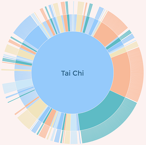
(As a detour, to understand the scope of what my training set covers, I’ve previously made a visualisation of this set of data, which will give you a quick overview. We’ll come back to this later.)

Once that was saved, I ran a similar command to the one detailed in the docker-torch-rnn instructions, but swapped in my file and directory names to the ones I wanted instead of their sample data. I used this:

python scripts/preprocess.py --input_txt data2/activities.txt --output_h5 data2/activities.h5 --output_json data2/activities.json

What this does is to run an input (signalled by input_txt) through the preprocess.py file within the scripts folder (this is part of the Docker image and you don’t need to add it). This will generate two output files - an h5 file, and a JSON file. We’re doing this by using the Python programming language, but again as we’re running the command from within the predefined Docker image we don’t need to install Python ourselves.

If all goes to plan, you should see something like this in your command prompt:

Total vocabulary size: 71
Total tokens in file: 12760
Training size: 10208
Val size: 1276
Test size: 1276
Using dtype

Now we should have everything that we need. You can check for yourself by navigating to the directory that our training file was in (remember I called mine ‘data2’ but yours may be different) by using the following:

cd data2

This changes our location into the directory called data2.

ls

This is the command to list everything in that directory.

You should see three files - the original text file, an .h5 version, and a .json version.

To return to the location we were before, type in:

cd ..

This takes us back out of the directory we’d gone into.

Training

Now that we have our training set in the right format it’s time to put it to use. Right now, you want to be boiling your kettle, by the way.

This next part was my second main stumbling point. The example in the documentation gives a command that errored for me. With some searching, I identified that it was because there’s an un-specified default for batch_size on that command, which as standard batches up your training data into 50s. Mine was breaking because I didn’t have enough training data for batches of that size to work. I settled on 10 for my first set, which worked. There’s some quite nice explanations of batches here.

There are actually quite a few different parameters that you can play around with, listed in the documentation for training, each of which may need to be considered depending on your own data. For my first pass, I just used the following:

th train.lua -batch_size 10 -input_h5 data2/activities.h5 -input_json data2/activities.json -gpu -1

What this is doing is running the training programme with the parameters that we’ve defined (things like batch size) and the input files that we’d previously created with the preprocessing step. The final flag of -gpu -1 is to make sure that we’re running in CPU as opposed to GPU mode based on the previous decision on this front (see CPU vs GPU section above).

Ok! So once you’ve picked all of the different parameters that apply, run your command, grab your boiled kettle, and make a cup of tea. This may take a while depending on the size of your training set.

Time passes…

One the command finishes running, you may feel slightly underwhelmed. Where’s my amusing output?

The answer lies within yet more generated files. If you want to check they’re there, you can do a similar process to the one I detailed at the end of the pre-processing section, but this time using:

cd cv

cv is the directory that your generated files will live in. These take the form of checkpoint files that will be generated to chunk up output - as you can imagine, some larger sets may have a lot of output!

It’s worth having a look, as I’m not sure yet on the logic behind what gets created. With my initial small sets I had only one checkpoint (two files - checkpoint_1000.json and checkpoint_1000.t7). You’ll need to see what your output was, as you’ll need a filename for the next step.

To see what’s been generated, we need to run one final command. Remember to adapt the path to the checkpoint file based on both the names of the files generated, and your location (i.e. if you’re still in the cv folder you’ll need to go back up a level to successfully run the below). My command was the following:

th sample.lua -checkpoint cv/checkpoint_1000.t7 -gpu -1

As before, the -gpu -1 flag is important if you’re running in CPU mode.

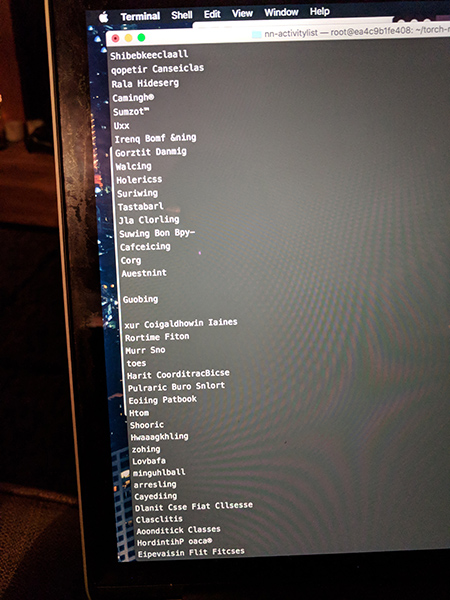
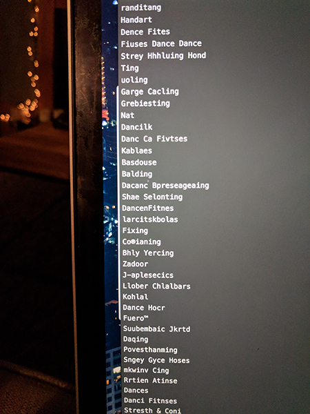
Et voila! You should hopefully see many amusing words running down your screen.

My output

My first run through was not perfect, but there was still something a little bit magical about it. The output was lots of made up words, but within it there were some gems that could actually be viable activity names. A lot of them were dance-centric, which reflects the high-number of dancey terms within the list - you can again see this using the visualisation.

Here’s some output.

Since then I’ve written a little harvesting programme to trawl through all of the actual OpenActive data sets (rather than just activity values), which cover real physical activity sessions across the country. I grabbed over 30,000 of them, and generated some session titles. I’ve also been tweaking the parameters from this original example to understand a bit more about how to get the best results, but all that can wait for another blog post. Until then, I hope that you’ve found this interesting, and let me know if you use it to create your own nonsense!